Flow technique deconstruction
Introduction
The animation When I first saw this animation, I was in awe. Never seen anything like it, beautiful and unique! The original author is Terebus Volodymyr. You can find the original work here. I immediately wanted to know how it worked, but the code was hard to read. Instead of leaving it at that, I annotated the whole thing so I could completely understand every single line of code. The goal here was to cut the codebase up into reusable functions and techniques to add them to my generative-art toolbox, so I can play around with them myself.
This post describes how the animation works, it does so by deconstructing the application. First, I'll extract all motion-related techniques used in this animation. Secondly, I'll take a look at the presentation of the particles and at the end, I'll bring everything back together. If you want, you can also read my annotations on his original code; the annotated code version of the animation.
Deconstruction of motion
To understand what he was doing, I annotated the code. Even though the code is very unstructured, I was still able to deconstruct it into individual techniques. Some of these techniques were completely new to me, and I'll definitely be using some of them in upcoming projects. First, I'll describe how the animation works in a global manner.
There are three sets of points, the first set describes a shape, for example, a square, a circle or a heart. I call this set the `originPoints` set, this set never changes throughout the entirety of the animation. The second set is a set of particles, each particle has a color, a position and a few parameters that affect their change in position over time. In addition to these simple parameters, each particle also has a `target` associated with it, these targets can be found in the third set `targetPoints`. The targetPoints are initially set to be the same as the `originPoints`, but get scaled up and down based on time.
Now, to get the brilliant motions as seen in the animation, three things are at play.
Click and drag the target around to see the spring behavior in action First of all, each particle moves relative to its target according to a spring equation.
Notice how the target changes Secondly, at every frame, there's a small chance that the particle gets a new target, completely changing its course.
The pulsating behavior of the targets Thirdly, the targets move on every frame, based on a "pulsating" scaling.
To get the trails, Terebus also thought of something quite unique. I was familiar with two way to do trails. The first option is to not completely clear the canvas on every frame, but to clear it with a highly transparent color, 'rgba(0, 0, 0, 0.1)' is commonly used. The second option is to keep track of a particle's previous position in a `positionHistory` kind of array.
Tracking behavior, move the target by dragging your mouse
Terebus uses the transparent clear technique, together with something that's close to the second, but instead of keeping track of the particle's previous position, he uses a cascading "tracking" movement. The tracking movement is a type of movement where on every frame, a particle moves n% to a target, this creates a smooth movement towards the target.
Move the target by dragging with your mouse What he does to create the trails is quite brilliant, the trail of trace-particles is 50 particles long, then, for each particle in the set, it uses the before-mentioned tracking behavior to move towards the next particle in the set. Feel for yourself how this motion works.
Illustration of the three different phases Apart from using prettier colors and more particles, there is one more thing that Terebus did. The pulsating behavior that I illustrated above is linear, in the original animation however, you could see a few different phases of the animation. There are three phases.
- Phase A, expanding. In this phase, the shape grows at a normal pace to its largest size. The background of the animation is blue during this phase.
- Phase B, expanded. In this phase, time is slowed down by a factor five compared to phase A, such that the shape stays at its most expanded for some time. The background of the animation is green during this phase.
- Phace C, imploding. In this phase, time is accelerated by a factor 9, to quickly implode the shape to a singularity. The background of the animation is red during this phase.
Illustration of the three different phases
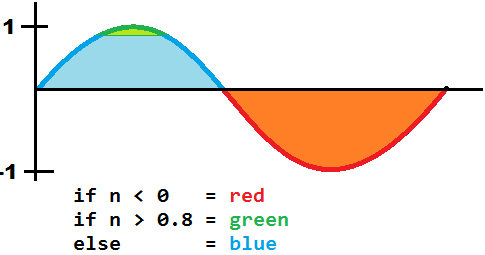 This effect is achieved by checking for different thresholds on the sine of time. A different perspective is to look at the actual sine wave, the colors of the sine wave describe the phases.
Note, if you know a better way to plot sine waves like these, please let me know. Paint is not a great program for this.
Deconstruction of color
The individual programs might give you an idea of what's going on underneath the surface, but you cannot see how these pulsating, trailing blobs result in the imagery as seen above.
Trajectory of a single particle First, let's look at the trajectory a particle takes in the final application. Note, this is without pulsing.
Trajectory of a single particle with trail Next, add the trail
Trajectory of a single particle with trail and color Give the particles the right color, and utilize the transparent-clearing technique, and we're done! All the difference between this one and the actual application is that there is only one particle, and the heart in this one doesn't pulse. Also, I've given the particle a random starting position, as is the case in the original application.
Reconstruction
The end!
In the end, we've learned the set of techniques Terebus applied to get to his result. I've italicized the techniques that were new and very insightful to me.
-
Movement
- Spring equations
- Chain of tracking equations -- trails
- Pulsing
- Sine wave thresholds -- abrupt movement and pulsing
- Target switching Color
- Transparent clearing
- Drawing an entire trail
I hope this was either informative or enjoyable for you. I'm planning on doing more of these articles, where I'll be deconstructing (deceptively?) complex pieces of generative art.